This paper proposes new six formulas allowing to calculate all roots of sixth degree polynomial equation nearly in parallel while including the use of radical expressions, which is extending a new engineering methodology to solve polynomial equations of nth degree where the value of n can exceed five. This methodology is based on developing the roots of nth degree polynomial equation according to a distributed structure of radical terms, where each term is built by multiplying two radicals presenting the roots of polynomial equations with inferior degrees. This distributed structure of terms is allowing them to neutralize each other during multiplications, which forward calculations toward eliminating radicalities, suppressing complex terms and reducing degrees. As a result, this paper is proposing new two theorems solving sixth degree polynomial equation in complete forms while relying on two different approaches built on the same engineering methodology of roots architecting, which allow calculating solutions nearly in parallel. This engineering methodology is scalable to solve higher degrees of polynomial equations while extending the same distributed architecture of terms whereas re-engineering the expressions of included sub-terms in order to manifest the same outcomes of reciprocal neutralization, radicality suppression and degrees reduction during calculations. Therefore, this paper is also presenting the engineered requirements and techniques along with details in order to scale the used methodology by projecting it on nth degree polynomial equations where the possibility of calculating the values of all roots nearly in parallel whereas the polynomial degrees can exceed the quantic form. The new proposed engineering methodology in this paper is listing all necessary logic, techniques and formulas to solve nth degree polynomial equations in general forms stage-by-stage while relying on the use of radical expressions, which will scale the results of this paper toward solving highly complex equations.
| Published in | American Journal of Applied Mathematics (Volume 13, Issue 1) |
| DOI | 10.11648/j.ajam.20251301.16 |
| Page(s) | 73-94 |
| Creative Commons |
This is an Open Access article, distributed under the terms of the Creative Commons Attribution 4.0 International License (http://creativecommons.org/licenses/by/4.0/), which permits unrestricted use, distribution and reproduction in any medium or format, provided the original work is properly cited. |
| Copyright |
Copyright © The Author(s), 2025. Published by Science Publishing Group |
New Formulas, New Six Roots, New Engineered Theorems, Sixth Degree Polynomial Equation, Solving Sixth Degree Equation, Solving Nth Degree Polynomial Equations
 does help Ferrari’s solution to solve quartic equations by reducing their expressions from the fourth degree to the second degree, but it does not directly help to properly define the four roots of any quartic equation. Therefore, when having a fourth-degree polynomial equation in general form, it is necessary to conduct further calculations to determine its four roots while relying on the solution of Ferrari Lodovico.
  degree equations; such as by using specific radical expressions under the form
  where the values of n can vary in the range
  , …, etc.
  of
of  degree by relying on its transformation into a reduced polynomial form
  with fewer terms by scaling the proposed idea of Descartes; in which a polynomial of
  degree is practically reducible by removing its term in the degree
  . The projection of this published method on quantic forms of polynomial equations is presented with more details in
  , can be solved by factorization or by relying on variable change, but other sixth degree equations in complete forms could not be solved over history
  , which will be multiplied by each other during calculations.
  where
where  by presenting it as
  .
.  to eliminate the term of degree
  from a polynomial equation of nth degree
  when
when  is an odd value or when this elimination is simplifying calculations.
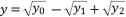
  should be expressed according to a sum of simple radical terms
  when the degree of polynomial equation is equal four.
  should be expressed according to a multiplication of at least two different sub-terms
  when the degree of polynomial equation is surpassing four.
  in the distributed structure of a root
  should appear in multiple distributed terms in order to allow further factorizations.
  in the distributed structure of terms
  should be presented according to a radical expression of cubic root, quadratic root or a constant.
 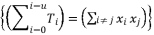 should include a sub-term
  presented according to a radical expression of cubic root where
 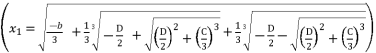 .
.  presented according to radical expressions of quadratic roots where
 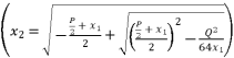 and
and 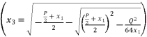 .
.  expressed by using included sub-terms in the distributed structure of root where
  .
.  expressed by using included sub-terms in the distributed structure of root where
 expressed by using included sub-terms in the distributed structure of root where
 expressed by using included sub-terms in the distributed structure of root where
  .
.  to be presented as
  .
.  to be presented as
  .
.  to be presented as
  .
.  and the expression
  in order re-express the polynomial equation
  to be represented as
  where
where  .
.  , we adopt a constant value
  where
where  is expressed in function of
  ; in order to converge calculations during the process of equations solving.
  in the distributed structure of a root
  should also be used in the calculation of all other roots by changing signs of these sub-terms whereas exploiting the involved coefficients in the polynomial equation.
  nearly in parallel.
  . We are proposing four solutions for
  , four solutions for
  and four solutions for
  .
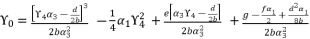
.  , which is presented in (eq.17), and by using
  ,
,  and
and  shown in (eq.6).
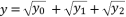
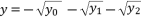
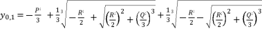
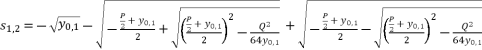
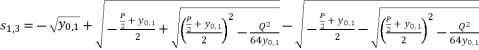
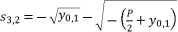
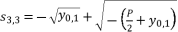
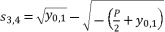
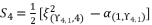
  , has four solutions:
  (1)
(1)  presented in the expression (eq.35);
  presented in the expression (eq.36);
  presented in the expression (eq.37);
  presented in the expression (eq.38).
  presented in the expression (eq.39);
  presented in the expression (eq.40);
  presented in the expression (eq.41);
  presented in the expression (eq.42).
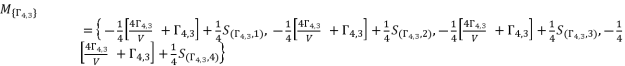
  presented in the expression (eq.43);
  presented in the expression (eq.44);
  presented in the expression (eq.45);
  presented in the expression (eq.46).
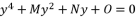
  , we have the next form:
  (2)
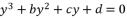
(2)  is expressed as shown in (eq.3):
  (3)
(3)  with supposed expression in (eq.3) to reduce the form of presented polynomial in (eq.2). Thereby, we have the presented expression in (eq.4).
  (4)
(4)  (5)
(5)  (6)
(6)  ; expressions (eq.7) and (eq.8):
  :
:  (7)
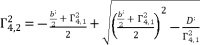
(7)  :
:  (8)
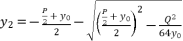
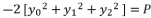
(8)  and
and  successively, in condition of
  . Those expressions of
  and
and  are based on quadratic solutions.
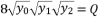
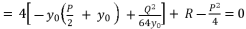
 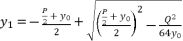 (9)
(9)  (10)
(10)  and
and  :
:  (11)
(11)  :
:  (12)
(12)  :
:  (13)
(13)  with the expression (eq.7) where we suppose
  , and we replace P and Q with their shown expressions in (eq.11) and (eq.12):

 (14)
(14)  , Cardano's solution is as follow:
 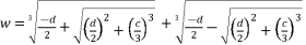 (15)
(15)  , we use the form
  and we suppose
  and
and  to express the cubic solution as follow:
 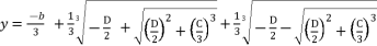 (16)
(16)  in (eq.17),
  in (eq.18) and
  in (eq.19), where
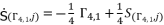
  ,
,  and
and 
 (17)
(17)  ,
,  and
and  are as follow:
 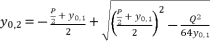 (18)
(18)  (19)
(19)  takes the value
  , the value of
  is equal to the shown value of
  in (eq.9), and the value of
  is equal to the shown value of
  in (eq.10).
  which respect the proposition
  when
when  , and they give the same results of calculations toward having the shown third degree polynomial in (eq.14). Thereby, they give the same values for roots
  and
and  . These three expressions are
  ,
,  and
and  .
.  are as shown in (eq.20), (eq.21), (eq.22) and (eq.23).
  (20)
(20)  (21)
(21)  (22)
(22)  (23)
(23)  which respect the proposition
  when
when  , and they give the same third degree polynomial shown in (eq.14) after calculations. These three expressions are
 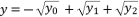 ,
,  and
and  .
.  are as shown in (eq.24), (eq.25), (eq.26) and (eq.27).
  (24)
(24)  (25)
(25)  (26)
(26)  (27)
(27) 
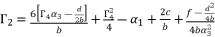
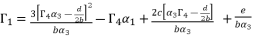
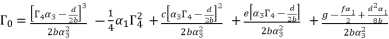
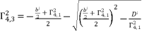
 is as shown in (eq.28) where
  and
and  , whereas
  and
and  are as shown in (eq.29) and (eq.30).
  (28)
(28)  (29)
(29)  (30)
(30)  or
or  , and having the intersection between the forms (eq.7) and (eq.8) for Q=0
  , there are four solutions for the polynomial equation shown in (eq.5) when Q=0 and they are as shown in (eq.31), (eq.32), (eq.33) and (eq.34).
 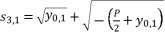 (31)
(31)  (32)
(32)  (33)
(33)  (34)
(34)  in (eq.17) to
  , the values of
  in (eq.18) and
  in (eq.19) are equal to the shown values of
  in (eq.9) and (
  in (eq.10) respectively. Thereby, even when we replace the value of
  in the expressions of proposed solutions by the values of
  or
or  , the results are only redundancies of proposed solutions, because the value of
  in the precedent expressions and in the proposed solutions is as follow:
 where
where  is the unknown variable in polynomial equation (eq.5). By using expressions (eq.6) and (eq.17) for
  , the solutions for equation (eq.1) are as shown in (eq.35), (eq.36), (eq.37) and (eq.38).
  (35)
(35)  (36)
(36)  (37)
(37)  (38)
(38)  while relying on expressions (eq.6) and (eq.17) for
  , the proposed solutions for equation (eq.1) are as shown in (eq.39), (eq.40), (eq.41) and (eq.42).
  (39)
(39)  (40)
(40)  (41)
(41)  (42)
(42)  while relying on expressions (eq.6) and (eq.28) for
  , the proposed solutions for equation (eq.1) are as shown in (eq.43), (eq.44), (eq.45) and (eq.46).
 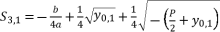 (43)
(43)  (44)
(44)  (45)
(45)  (46)
(46)  (47)
(47)  (48)
(48)  (49)
(49)  (50)
(50)  , whereas supposing
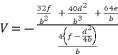
  is the solution for fourth degree polynomial equation in (eq.50) by using Theorem 1 and relying on the expression
  The variable
  is defined as shown in (eq.51) where
  is presented in (eq.52) and
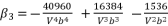
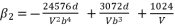
  is the solution for the polynomial equation (eq.53), which relies on the coefficients (eq.54), (eq.55), (eq.56) and (eq.57). The shown coefficients in (eq.54), (eq.55), (eq.56) and (eq.57) are expressed by using the constant
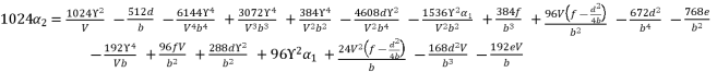
  which is presented in (eq.58). The coefficients
  ,
,  ,
,  and
and  of quartic equation (eq.50), which is used to calculate
  , are determined by using the shown expressions in (51), (eq.59), (eq.60) and (eq.61) while using calculated values of
  and
and  . As a result, we have twelve calculated values as potential solutions for sixth degree polynomial equation shown in (eq.48), where many of them are only redundancies of others, because there are only six official solutions to determine.
  (51)
(51)  (52)
(52)  (53)
(53)  (54)
(54)  (55)
(55)  (56)
(56)  (57)
(57)  (58)
(58)  (59)
(59)  (60)
(60) 
 (61)
(61)  (62)
(62)  (63)
(63)  with its proposed value in (eq.62), in order to end by calculations to the reduced form shown in (eq.50).
  (64)
(64)  (65)
(65)  (66)
(66)  (67)
(67)  (68)
(68)  (69)
(69)  (70)
(70)  (71)
(71)  in (eq.64),
  in (eq.65),
  in (eq.66),
  in (eq.67),
  in (eq.68),
  in (eq.69) and
  in (eq.70), to have the fourth degree polynomial shown in (eq.71) where the values of coefficients are as follow:


 to simplify its expression. As a result, we have the shown equation in (eq.50) where the values of coefficients are as follow:

 for fourth degree polynomial equation in simple form shown in (eq.5), whereas the solution for fourth degree polynomial equation in complete form is expressed as
 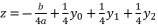 .
.  with
with  in order to reduce the form of quartic equation from expression (eq.50) to expression (eq.72), where the values of coefficients are as shown in (eq.73).
 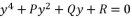 (72)
(72)  (73)
(73)  is as shown in (eq.63), the principal proposed expressions for the solutions are
 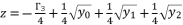 when
when  and
and  ; where
 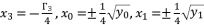 and
and  . These two principal expressions are sufficient to conduct the calculations of proof, and then generalize the results by using the other expressed forms of solutions in Theorem 1.
  with their values in function of
  in order to have the expressions of
  in (eq.74),
  in (eq.75) and
  in (eq.76).
 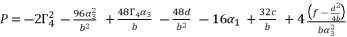 (74)
(74) 
 (75)
(75) 
 (76)
(76)  ,
,  and
and  are as shown in (eq.77), (eq.78) and (eq.79) successively.
  (77)
(77)  (78)
(78) 
 (79)
(79)  , whereas we have a group of only three equations to solve
  where all of them are dependent on the value of
  . Thereby, the next step is about using the appropriate logic of analysis and calculation to find the value of
  while taking advantage of the fact that having a group of four variables enables us to solve four equations.
  in (eq.76), and find a way to determine the value of
  , we suppose that
  where
where  . As a result, we have the shown expression in (eq.80).
  (80)
(80)  has a constant value. Therefore, in the rest of calculation, we will replace
  by the constant
  , which is shown in (eq.58).
  to simplify its expression, along using the expression of
  , we have
  .
.  in (eq.74) and (eq.77), which we use to define the shown value of
  in (eq.82).
  (81)
(81)  (82)
(82)  in (eq.76) and (eq.79).
 (83)
(83) 
 (84)
(84)  and then express
  as shown in (eq.85) where we rely on replacing
  with its constant value
  , which is presented in (eq.80).
 (85)
(85) 

 (86)
(86)  with its shown expression in (eq.82), and then we assemble terms of equation (eq.86) in function of degrees, in order to have the expression (eq.88) where coefficients are presented in (eq.54), (eq.55), (eq.56) and (eq.57).
  (87)
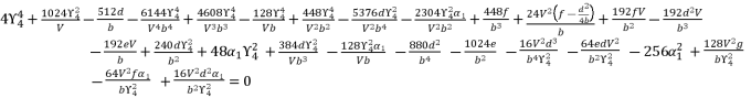
(87)  (88)
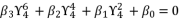
(88)  whereas adopting
  , we eliminate the root zero as solution for polynomial equation (eq.88) and we use the cubic solution to solve the polynomial equation
 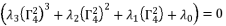 , because all coefficients are expressed only in function of
  ,
,  ,
,  ,
,  ,
,  and the constant
  . As a result, we have six possible values for
  as solutions for polynomial equation shown in (eq.53).
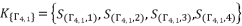
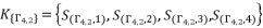
  is the group of solutions for shown equation in (eq.53), where these solutions are expressed as
  and
and  with
with  . The group of solutions
  is determined by relying on cubic root shown in (eq.90) and quadratic roots (eq.91) and (eq.92).
  (89)
(89)  ,
,  and
and  , whereas using the expressions (eq.54), (eq.55), (eq.56) and (eq.57). We suppose also that
 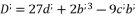 and
and  . The solutions
  ,
,  and
and  for shown equation in (eq.53) are as follow:
 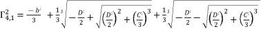 (90)
(90)  (91)
(91)  (92)
(92)  by using cubic solution and quadratic solutions, the following step consists of solving the polynomial equation shown in (eq.72).
  in (eq.74) and
  in (eq.76) are dependent on
  and
and  . The coefficient
  in (eq.82) is dependent on
  , whereas the coefficient
  shown in (eq.75) is dependent on
  and
and  . Therefore, we are going to use only
  ,
,  and
and  to calculate the potential values of
  because
  are going only to inverse the sign of coefficient
  and thereby inversing the signs of potential values of
  as solutions for polynomial equation shown in (eq.50), which will not influence the potential values of
  as solutions for sixth degree polynomial equation shown in (eq.48) because
 ,
,  and
and  for each value of
  from the group
  . Thereby, we have twelve values to calculate as potential solutions for the polynomial equation shown in (eq.72).
  from the group
  , we have three groups of potential solutions for polynomial equation shown in (eq.72), where each group is dependent on different value of
  . We express these groups of solutions as follow:
  .
.  (93)
(93)  (94)
(94)  (95)
(95)  ; as shown in (eq.96), (eq.97) and (eq.98). The values of
  , where
  and
and  , are from the expressed solutions in the groups (eq.93), (eq.94) and (eq.95).
 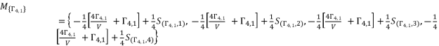 (96)
(96)  (97)
(97)  (98)
(98)  where
where  and
and  , in order to simplify the expressed values in (eq.96), (eq.97) and (eq.98). Thereby, we have three groups of values as potential solutions for sixth degree polynomial equation shown in (eq.48). These three groups are as shown in (eq.99), (eq.100) and (eq.101) where
  is as follow:
 is an extending of the shown expression of
  in (eq.82) by changing the value of
  , where
  belong to the group
  .
.  (99)
(99)  (100)
(100)  (101)
(101)  are the responsible of solution redundancies from one group to other.
  ,
,  and
and  , and then determining the six solutions for sixth degree polynomial equation shown in (eq.48), we propose the expressed values in (eq.102), (eq.103), (eq.104), (eq.105), (eq.106) and (eq.107) as the six official solutions for sixth degree polynomial equation shown in (eq.48).
  , whereas the fifth and sixth values are expressed by deduction using the expressions of quadratic roots. The useless redundancies of solutions are from one group to other; therefore, we choose the first four solutions from the same group
  .
.  where
where  and
and  from
from  . The variable
  is expressed as follow:
 is from the group
  shown in (eq.88) which contains the solutions for polynomial equation (eq.52). The values of
  , where
  , are the solutions for quartic equation (eq.50) and they are determined by using Theorem 1.
  (102)
(102)  (103)
(103)  (104)
(104)  (105)
(105)  (106)
(106)  (107)
(107)  where the coefficient of fifth degree part is equal zero imposes a problem of reduction to fourth degree.
  , where coefficients belong to the group of numbers ℝ and the coefficient of fifth degree part equal zero.
  to the expression
 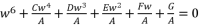 , and then we use the expression
  to induce a fifth degree part whereas eliminating the fourth degree part of concerned sixth degree polynomial.
  with
with  . The coefficients of equation (eq.108) are as expressed in (eq.109), (eq.110), (eq.111), (eq.112) and (eq.113).
  (108)
(108)  (109)
(109)  (110)
(110)  (111)
(111)  (112)
(112)  (113)
(113)  to the quartic equation shown in (eq.114), where coefficients belong to the group of numbers ℝ we first replace
  with
with  Then, the reduction from sixth degree to fourth degree is conducted by supposing
  , whereas supposing
  is the solution for fourth degree polynomial equation in (eq.114) by using Theorem 1 and relying on the expression
  . The variable
  is defined as shown in (eq.115) where
  is presented in (eq.119) and
  is the solution for the polynomial equation (eq.120), which relies on the coefficients (eq.121), (eq.122), (eq.123) and (eq.124). The shown coefficients in (eq.121), (eq.122), (eq.123) and (eq.124) are expressed by using the constant
  , which is defined in (eq.125). The coefficients
  ,
,  ,
,  and
and  of quartic equation (eq.114) are determined by using calculated value of
  and using the shown expressions in (eq.115), (eq.116), (eq.117) and (eq.118). The six proposed solutions for polynomial equation
  are as shown in (eq.136), (eq.137), (eq.138), (eq.139), (140) and (eq.141).
  (114)
(114)  (115)
(115)  (116)
(116)  (117)
(117)  (118)
(118)  (119)
(119)  (120)
(120)  (121)
(121)  (122)
(122)  (123)
(123)  (124)
(124)  (125)
(125)  where the fifth degree part is absent, we divide the polynomial on
  and then we use the expression
  in order to induce a fifth degree part and eliminate the fourth degree part. Then, by using the expression (eq.62), we reduce the resulted sixth degree polynomial (eq.108) to the quartic polynomial shown in (eq.126).
  (126)
(126)  in (eq.64),
  in (eq.65),
  in (eq.66),
  in (eq.67),
  in (eq.69) and
  in (eq.70) to express the fourth degree polynomial shown in (eq.126) where the values of coefficients are as follow:


 . The coefficients of polynomial (eq.114) are as follow:

 by replacing
  with
with  in the polynomial (eq.114). The coefficients
  ,
,  and
and  are as expressed in (eq.127), (eq.128) and (eq.129).
  (127)
(127)  (128)
(128)  (129)
(129)  in (eq.129), and find a way to determine the value of
  , we suppose that
  where
where  . As a result, we have the shown expression in (eq.130).
  (130)
(130)  ,
,  and
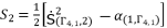
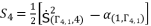
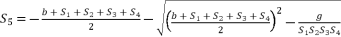
and  are as expressed in (eq.131), (eq.132) and (eq.133) respectively, whereas the resulted polynomial equation to determine the value of
  is as shown in (eq.134).
  (131)
(131)  (132)
(132)  (133)
(133)  (134)
(134)  in (eq.130) and we replace
  and
and  with their shown expressions in (eq.131) and (eq.133), in order to pass from equation (eq.134) to polynomial expression
  where coefficients are as presented in (eq.121), (eq.122), (eq.123) and (eq.124).
  shown in (eq.135) as a root for expressed equation in (eq.120), and then we determine the roots of quartic equation
  . Therefore, we start by calculating the values of
  ,
,  and
and  by replacing the variable
  with the value of
  , then we calculate the values of
  ,
,  and
and  , and finally we finish by using Theorem 1.
  and
and  , whereas using the expressions (eq.121), (eq.122), (eq.123) and (eq.124). We suppose also that
  and
and  . The solution
  for shown equation in (eq.120) is as follow:
 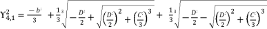 (135)
(135)  to calculate the values of
  ,
,  and
and  generates redundancies of roots for the sixth degree polynomial equation
  .
.  , which contains the four roots for quartic equation
  , by using Theorem 1.
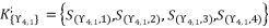
 , which is determined by relying on the group
  .
. 
 are as expressed in (eq.136), (eq.137), (eq.138), (eq.139), (140) and (eq.141). The expressions
  ,
,  ,
,  and
and  present the calculated roots for quartic equation (eq.114) by using Theorem 1.
  is calculated by using the shown expression in (eq.135). We use the expression (eq.131) to calculate the value of
  ; thereby, its value is as follow:
 (136)
(136)  (137)
(137)  (138)
(138)  (139)
(139)  (140)
(140)  (141)
(141)  where the fifth-degree part is absent, which is essential to reduce sixth degree polynomial equation to quartic equation. The third theorem is also distinguished by eliminating the fourth-degree part of concerned sixth degree polynomial, in order to reduce the amount of calculations.
 | [1] | Cardano, G. Artis Magnae, Sive de Regulis Algebraicis Liber Unus, 1545. English transl.: The Great Art, or The Rules of Algebra. Translated and edited by Witmer, T. R. MIT Press, Cambridge, Mass, 1968. |
| [2] | Dumit, D. S. Foote, R. M. 2004. Abstract algebra. John Wiley, pp. 606-616. |
| [3] | Osler, T. J. 2001. Cardan polynomials and the reduction of radicals, Mathematics Magazine, vol. 47, no. 1, pp. 26-32. |
| [4] | Euler, L. De formis radicum aequationum cuiusque ordinis coniectatio, 1738. English transl.: A conjecture on the forms of the roots of equations. Translated by Bell, J. Cornell University, NY, USA, 2008. |
| [5] | S. Janson, Roots of polynomials of degrees 3 and 4, 2010. |
| [6] | René, D. The Geometry of Rene Descartes with a facsimile of the 1st edition, Courier Corporation, 2012. |
| [7] | Lagrange, J. L. Réflexions sur la résolution algébrique des équations, in: ouvres de Lagrange, J. A. Serret ed & Gauthier-Villars, Vol. 3, pp. 205-421, 1869. |
| [8] | Faucette, W. M. 1996. A geometric interpretation of the solution of the general quartic polynomial, Amer. Math. Monthly, vol. 103, pp. 51-57. |
| [9] | Bewersdor, J. Algebra fur Einsteiger, Friedr. Vieweg Sohn Verlag. English transl.: Galois Theory for Beginners. A Historical Perspective, 2004. Translated by Kramer, D. American Mathematical Society (AMS), Providence, R. I., USA, 2006. |
| [10] | Helfgott, H. Helfgott, M. A modern vision of the work of cardano and ferrari on quartics. Convergence (MAA). |
| [11] | Rosen, M. 1995. Niels hendrik abel and equations of the fiffth degree, American Mathematical Monthly, vol. 102, no. 6, pp. 495-505. |
| [12] | Garling, D. J. H. Galois Theory. Cambridge Univ. Press, Mass., USA, 1986. |
| [13] | Grillet, P. Abstract Algebra. 2nd ed. Springer, New York, USA, 2007. |
| [14] | van der Waerden, B. L. Algebra, Springer-Verlag, Berlin, Vol. 1, 3rd ed. 1966. English transl.: Algebra. Translated by Schulenberg J. R. and Blum, F. Springer-Verlag, New York, 1991. |
| [15] | Shmakov, S. L. 2011. A universal method of solving quartic equations, International Journal of Pure and Applied Mathematics, vol. 71, no. 2, pp. 251-259. |
| [16] | Fathi, A. Sharifan, N. 2013. A classic new method to solve quartic equations,” Applied and Computational Mathematics, vol. 2, no. 2, pp. 24-27. |
| [17] | Tehrani, F. T. 2020. Solution to polynomial equations, a new approach, Applied Mathematics, vol. 11, no. 2, pp. 53-66. |
| [18] | Nahon, Y. J. 2018. Method for solving polynomial equations, Journal of Applied & Computational Mathematics, vol. 7, no. 3, pp. 2-12. |
| [19] | Tschirnhaus, E. A. method for removing all intermediate terms from a given equation, THIS BULLETIN, vol. 37, no. 1, pp 1-3. Original: Methodus auferendi omnes terminos intermedios ex data equatione, Acta Eruditorium vol. 2, pp. 204-207, 1683. |
| [20] | Adamchik, V. S. Jeffrey, D. J. 2003. Polynomial transformations of tschirnhaus, bring and jerrard, ACM SIGSAM Bulletin, vol. 37, no. 3, pp. 90-94. |
| [21] | Lazard, D. Solving quintics in radicals. In: Olav Arnfinn Laudal, Ragni Piene, The Legacy of Niels Henrik Abel. 1869, pp. 207-225. Springer, Berlin, Heidelberg. |
| [22] | Dummit, D. S. 1991. Solving solvable quintics, Mathematics of Computation, vol. 57, no. 1, pp. 387-401. |
| [23] | Samuel, BB. 2017. On Solvability of Higher Degree Polynomial Equations, Journal of Applied Science and Innovations, vol. 1, no. 2. |
| [24] | Samuel, BB. The General Quintic Equation, its Solution by Factorization into Cubic and Quadratic Factors, Journal of Applied Science and Innovations, vol. 1, no. 2, 2017. |
| [25] | Pesic, P. 2004. Abel’s Proof: An Essay on the Sources and Meaning of Mathematical Unsolvability, MIT Press. |
| [26] | Wantzel, P. L. 1845. Démonstration de l'impossibilité de résoudre toutes les équations algébriques avec des radicaux, J. Math. Pures Appl., 1re série, vol. 4, pp. 57-65, |
| [27] | Larbaoui, Y. New Theorems and Formulas to Solve Fourth Degree Polynomial Equation in General Forms by Calculating the Four Roots Nearly Simultaneously. American Journal of Applied Mathematics. vol. 11(6): 95-105. |
| [28] | Larbaoui, Y. New Theorems Solving Fifth Degree Polynomial Equation in Complete Forms by Proposing New Five Roots Composed of Radical Expressions. American Journal of Applied Mathematics. Vol2. 1: 9-23. |
APA Style
Larbaoui, Y. (2025). New Six Formulas of Radical Roots Developed by Using an Engineering Methodology to Solve Sixth Degree Polynomial Equation in General Forms by Calculating All Solutions Nearly in Parallel. American Journal of Applied Mathematics, 13(1), 73-94. https://doi.org/10.11648/j.ajam.20251301.16
ACS Style
Larbaoui, Y. New Six Formulas of Radical Roots Developed by Using an Engineering Methodology to Solve Sixth Degree Polynomial Equation in General Forms by Calculating All Solutions Nearly in Parallel. Am. J. Appl. Math. 2025, 13(1), 73-94. doi: 10.11648/j.ajam.20251301.16
AMA Style
Larbaoui Y. New Six Formulas of Radical Roots Developed by Using an Engineering Methodology to Solve Sixth Degree Polynomial Equation in General Forms by Calculating All Solutions Nearly in Parallel. Am J Appl Math. 2025;13(1):73-94. doi: 10.11648/j.ajam.20251301.16
@article{10.11648/j.ajam.20251301.16,
  author = {Yassine Larbaoui},
  title = {New Six Formulas of Radical Roots Developed by Using an Engineering Methodology to Solve Sixth Degree Polynomial Equation in General Forms by Calculating All Solutions Nearly in Parallel
},
  journal = {American Journal of Applied Mathematics},
  volume = {13},
  number = {1},
  pages = {73-94},
  doi = {10.11648/j.ajam.20251301.16},
  url = {https://doi.org/10.11648/j.ajam.20251301.16},
  eprint = {https://article.sciencepublishinggroup.com/pdf/10.11648.j.ajam.20251301.16},
  abstract = {This paper proposes new six formulas allowing to calculate all roots of sixth degree polynomial equation nearly in parallel while including the use of radical expressions, which is extending a new engineering methodology to solve polynomial equations of nth degree where the value of n can exceed five. This methodology is based on developing the roots of nth degree polynomial equation according to a distributed structure of radical terms, where each term is built by multiplying two radicals presenting the roots of polynomial equations with inferior degrees. This distributed structure of terms is allowing them to neutralize each other during multiplications, which forward calculations toward eliminating radicalities, suppressing complex terms and reducing degrees. As a result, this paper is proposing new two theorems solving sixth degree polynomial equation in complete forms while relying on two different approaches built on the same engineering methodology of roots architecting, which allow calculating solutions nearly in parallel. This engineering methodology is scalable to solve higher degrees of polynomial equations while extending the same distributed architecture of terms whereas re-engineering the expressions of included sub-terms in order to manifest the same outcomes of reciprocal neutralization, radicality suppression and degrees reduction during calculations. Therefore, this paper is also presenting the engineered requirements and techniques along with details in order to scale the used methodology by projecting it on nth degree polynomial equations where the possibility of calculating the values of all roots nearly in parallel whereas the polynomial degrees can exceed the quantic form. The new proposed engineering methodology in this paper is listing all necessary logic, techniques and formulas to solve nth degree polynomial equations in general forms stage-by-stage while relying on the use of radical expressions, which will scale the results of this paper toward solving highly complex equations.
},
 year = {2025}
}
TY  - JOUR
T1  - New Six Formulas of Radical Roots Developed by Using an Engineering Methodology to Solve Sixth Degree Polynomial Equation in General Forms by Calculating All Solutions Nearly in Parallel

AU  - Yassine Larbaoui
Y1  - 2025/02/21
PY  - 2025
N1  - https://doi.org/10.11648/j.ajam.20251301.16
DO  - 10.11648/j.ajam.20251301.16
T2  - American Journal of Applied Mathematics
JF  - American Journal of Applied Mathematics
JO  - American Journal of Applied Mathematics
SP  - 73
EP  - 94
PB  - Science Publishing Group
SN  - 2330-006X
UR  - https://doi.org/10.11648/j.ajam.20251301.16
AB  - This paper proposes new six formulas allowing to calculate all roots of sixth degree polynomial equation nearly in parallel while including the use of radical expressions, which is extending a new engineering methodology to solve polynomial equations of nth degree where the value of n can exceed five. This methodology is based on developing the roots of nth degree polynomial equation according to a distributed structure of radical terms, where each term is built by multiplying two radicals presenting the roots of polynomial equations with inferior degrees. This distributed structure of terms is allowing them to neutralize each other during multiplications, which forward calculations toward eliminating radicalities, suppressing complex terms and reducing degrees. As a result, this paper is proposing new two theorems solving sixth degree polynomial equation in complete forms while relying on two different approaches built on the same engineering methodology of roots architecting, which allow calculating solutions nearly in parallel. This engineering methodology is scalable to solve higher degrees of polynomial equations while extending the same distributed architecture of terms whereas re-engineering the expressions of included sub-terms in order to manifest the same outcomes of reciprocal neutralization, radicality suppression and degrees reduction during calculations. Therefore, this paper is also presenting the engineered requirements and techniques along with details in order to scale the used methodology by projecting it on nth degree polynomial equations where the possibility of calculating the values of all roots nearly in parallel whereas the polynomial degrees can exceed the quantic form. The new proposed engineering methodology in this paper is listing all necessary logic, techniques and formulas to solve nth degree polynomial equations in general forms stage-by-stage while relying on the use of radical expressions, which will scale the results of this paper toward solving highly complex equations.

VL  - 13
IS  - 1
ER  -
Department of Electrical Engineering, Université Hassan 1er, Settat, Morocco
Information


 , and by using the expressions of
  in (eq.
 , and by using the expressions of
  in (eq.
 , and by using the expressions of
  in (eq.
 ,
,  and
and  where
where  and
and  .
.  with its shown expression in (eq.
 with its shown expression in (eq.
 , whereas
  is from the group
  .
.